3D Graphics Systems Course - IMPA 2020

Professor Luiz Velho

Hallison Paz, 1st year PhD student

---

Rendering a Scene with a Differentiable Renderer

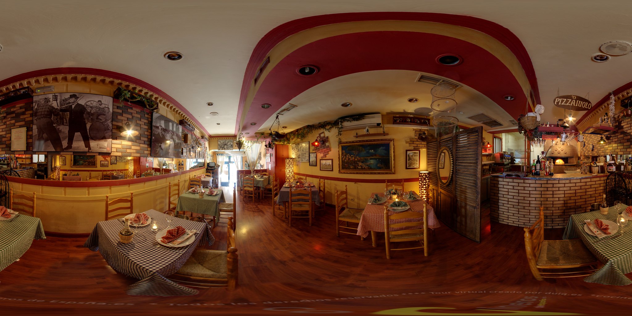
The objective of this 2nd assignment is to render a scene using the differentiable renderer implemented in PyTorch3D and exploit some capabilities of this system. We aim to render equirectangular panoramas, building a scene with a single sphere parameterized by latitude and longitude and setting the camera in the center of the sphere. You can find the full source code here.

Modeling the Scene

First of all, we need to compute the geometry and texture coordinates for a sphere. We decided to parameterize the sphere in terms of latitude and longitude coordinates, as well as use an equirectangular panorama as a bidimensional texture for the interior of the sphere. A valid concern about textures is the possibility of distortion due to the mapping; using this representation, we have an image and a natural map that takes into account the distortion of the surface.

Geometry and Texture Coordinates

For the geometry, we sample points uniformly as we increment the angles Phi and Theta in a spherical coordinate system. 0 <= Phi <= 2pi; 0 <= Theta < pi. As the texture has a boundary and the sphere has not, we must be careful to achieve a good and meaningful result. Our strategy for a good mapping was:

1. We don’t close the sphere in the poles. As we can see in line #2, we define an epsilon, so that Theta actually varies from epsilon to pi-epsilon and the vertices of the poles are sampled very close to each other, but are still considered different elements.

2. We duplicate the vertices located over the first meridian. For each parallel, we sample two vertices on the exact same location of the first sample, which is equivalent to consider that Phi belongs to the closed interval [0, 2PI]. We do that to simplify the computations of the texture reconstruction on the surface, as it can be done with a linear interpolation. Lines #19 to #25 implement this approach.

Mesh Triangulation

We triangulate the mesh by connecting vertices on adjacent parallels and meridians over the surface. We choose the order of the vertices such that each face has a clockwise (CW) winding order. This way, the normals point to the interior of the surface where we wish to locate our camera.

In the end of the function we convert the lists of data into PyTorch tensors, so we have a data structure compatible with the operations of the library.

Rendering the Scene

This tutorial in the PyTorch3D website shows how to set up a renderer to render a textured mesh. We used it as a starting point to our experiments.

Loading mesh data

The tutorial shows how to load an obj file and material data into memory to render a textured surface. Our first approach was to try to write the computed geometry of the mesh and texture information to an obj file and then, follow similar steps. However, we discovered that the library does not support saving a mesh with texture coordinates yet and it does not plan to add this feature soon. To solve this problem, we figured how to use the Texture class out of the source code.

Setting the scene parameters

On the first experiment, we tried to reproduce the tutorial steps to check if the texture data is fine and see what would be rendered. We can see part of the texture represented in a circular shape in an image that looks a little dark. This result seems fine as we are looking to the sphere from the outside and the normals of the faces points inward the surface.

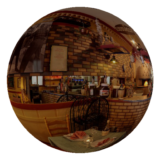
Câmera located at point [0.0, 0.0, 2.1] (outside)

After that, we moved the camera and the light source to the center of the sphere, decreasing the near clipping plane to 0.5 as the radius of the sphere is equal to 1.0. For our surprise the result was only a black screen.

We decided to put the camera outside the sphere again and render some intermediate images as we move the camera towards the center of the sphere.

Camera located at point [0.0, 0.0, 1.2] (outside)

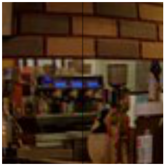
Camera located at point [0.0, 0.0, 0.9] (inside)

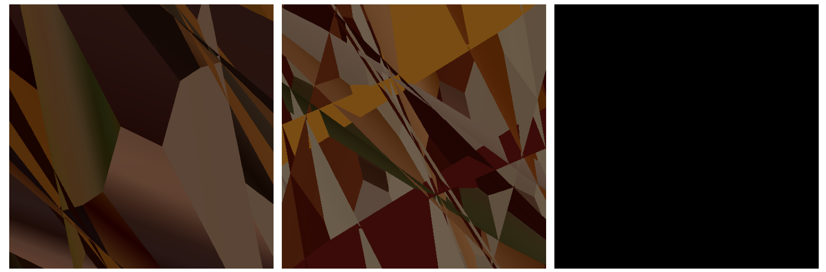
Cameras located at points [0, 0, 0.6] | [0, 0, 0.3] | [0, 0, 0.0] (inside)

As we can see, as soon as the camera enters the surface, the visualization gives an unexpected result. Setting the camera anywhere inside the sphere but the center, appears to show a distorted visualization where we can’t identify any object in the texture. In the center, we have a black screen, which we believe is a texture dependent result, based on further experiments that we’ll describe below.

Investigating the unexpected results

Rendering the Mesh in MeshLab

The first test we did to check if the error was in our computations, was to export the mesh and open it on MeshLab. We wrote a simple function to save an obj file with texture coordinates for vertices and we copied the material used in the cow mesh, changing only the image used as texture. In MeshLab, everything was ok, so we discarded a problem with our geometry.

Moving the câmera in the tutorial

We decided to take the original code of the tutorial and move the camera towards the inside of the cow mesh. We could observe the exact same problem. We discarded issues related to the winding order and normal orientation of the faces.

Toy texture

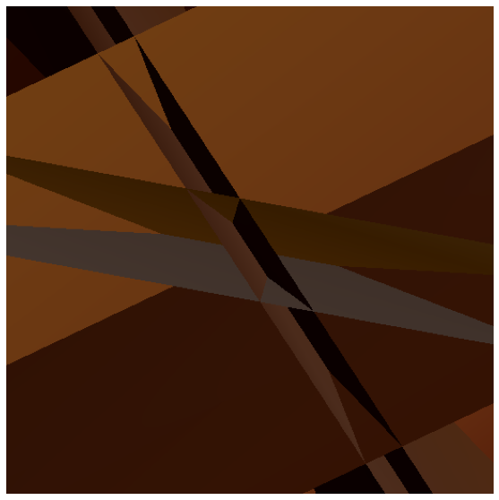
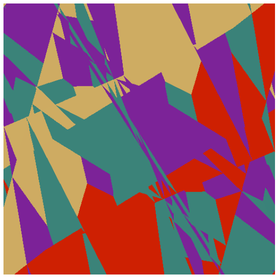
We decided to use a very simple texture, represented by 4 large rectangles in different colors, to try to investigate the problem by looking to the result.

Unfortunately, we couldn’t identify any pattern in the rendered image that could lead us to a solution. At first, we can see that some regions show patterns that resemble self-intersections or visibility problems related to depth sorting or face culling. We already checked that our mesh is correct and has no self-intersections, but to investigate visibility problems, we need to understand the details of this particular implementation.

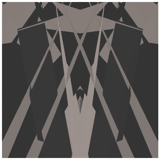
Camera located at point [0.0, 0.0, 0.3] (inside)

An interesting result was that, in this case, when we rendered the scene with the camera located in the center of the sphere, we didn’t get a black screen as we got using the first texture.

Camera located at point [0.0, 0.0, 0.0] (inside)

Changing Renderer Settings

We tried to explore different sets of the parameters faces_per_pixel, bin_size and max_faces_per_bin, but we could’t perceive any difference while rendering the “toy texture”. We tried both the coarse and coarse-to-fine rasterization as stated in the documentation.

raster_settings = RasterizationSettings(
   image_size=512, 
   blur_radius=0.0, 
   faces_per_pixel=1, 
   bin_size = None,  # this setting controls whether naive or coarse-to-fine rasterization is used
   max_faces_per_bin = None  # this setting is for coarse rasterization
)

Looking for alternatives renderers

We tried to use the library TensorFlow Graphics to render the mesh, but we couldn’t find information on how to render a textured mesh and it didn’t appear we could learn it and achieve the expected result on time.

Our second alternative was the Open Differentiable Renderer (OpenDR). Although this have a nice documentation of the examples, including a paper detailing how they achieved this result, we couldn’t run the examples. Later, we discovered it’s written in Python 2, which is deprecated as of 2020, and it’s not compatible with Python 3.

Finding a way to render the scene in another similar differentiable renderer system, can help us understand if it’s a problem related to the method or to the specific implementation in PyTorch3D. As we already spent a significant amount of time in this assignment, this point remains inconclusive for now.

Conclusion

Differentiable rendering is a powerful tool to unite the computer graphics and computer vision problems. Our primary goal was to render a 3D scene using the differentiable rendering implementation of PyTorch3D. Using equirectangular panoramas as bidimensional textures, we could render visually complex scenes using the very simple geometry of a sphere.

We managed to build on top of the knowledge acquired on the last assignment and model the desired scene using PyTorch3D, but the task of rendering showed itself more challenging than expected. We couldn’t achieve our primary goal as the rendering from cameras located inside a closed mesh resulted in distorted images.

We tried many different approaches to understand the unexpected behavior of the rendering and check which role our code played in this process. We could achieve the desired visualization using an external software with a regular rendering system based on rasterization, which helped us to validate our computed geometry and texture data. However, we still don’t know the real reason behind this unexpected result and we need to dive deeper in the implementation details to understand.